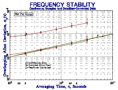
Nominal 1x10-11 Stability at t = 100 Seconds Shown by Green Lines
Plots Show Stability of Simulated Data Sets for Continuous, Sampled and Dead Time-Corrected Data
GAPS, OUTLIERS, DEAD TIME, AND UNEVEN SPACING
IN FREQUENCY
STABILITY DATA
W.J.
Riley, Hamilton Technical Services
ABSTRACT
Most measures of frequency stability (e.g. Allan and total variances, FFT power spectra) use continuous sets of equally spaced data. Actual clock data, however, often has gaps and outliers, may have dead time between measurements, and can be taken at uneven intervals. This paper offers suggestions regarding the analysis of such data using the Stable32 program for frequency stability analysis.
INTRODUCTION
Gaps in clock data are like death and taxes - one cannot totally avoid them. Gaps may occur as the result of missing data, or from outlier removal. While the latter should be rare, a string of gaps happens quite frequently in a long data record. This is where timetags can be a big help. They, along with the Stable32 Regularize function can automatically insert gaps as placeholders for the missing points. The analysis of clock data containing gaps must be done with care and common sense. If the objective is a stability analysis, that information can be obtained by ignoring the missing data and directly using the raw data. If, however, the objective is a plot of the phase or frequency record, or a determination of the frequency drift, then the time flow of the record is important, and gaps must be inserted for the missing points. The Stable32 data plotting and drift analysis functions can handle gaps without any problems. Performing a stability analysis for data with gaps is more complicated because of two factors (1) phase-frequency conversions and (2) variance calculations. The Stable32 phase-to-frequency conversion function will reproduce gaps in phase data as corresponding gaps in frequency data. Each phase gap section will cause one additional frequency gap because a missing phase point affects two adjacent frequency points (first differences of phase divided by tau). The Stable32 frequency-to-phase conversion is not as satisfactory because it produces a phase record that contains an interpolated portion that integrates the average frequency during the gap. This is necessary to provide phase continuity, but cannot be used for subsequent stability analysis. It is therefore better to start with phase data, analyze its stability, use its timetags to regularize it, plot the phase record, and then convert that corrected phase record to frequency data for drift analysis and plotting. An additional consideration is the implicit frequency-to-phase conversion that is often done during the stability analysis of frequency data. This is done because many of the phase data algorithms are much more efficient. Unfortunately, this can badly distort the results for frequency data having large gaps. Always examine the normal Allan deviation for such data - the other variances should be similar. The overlapping Allan deviation is also OK because a slower frequency data algorithm is used when gaps are present. So are the normal and overlapping Hadamard variances, which use direct frequency based calculations. The modified and total variances are subject to error for frequency data with gaps. Gaps can be filled with linearly interpolated values with the Fill function. This is done automatically for MTIE and several of the total variance functions where gap testing and bridging is impractical. Obviously, this is suspect for large gaps since fictitious data is used, and is particularly undesirable for uncorrelated (white) noise.
OUTLIERS
It is important to explain all outliers, thereby determining whether they are due to the measurement process or the device under test. An important first step is to correlate the bad point with any external events (e.g. power outages, equipment failures, etc.) that could account for the problem. Failures of the measurement system, frequency reference, or environmental control are often easier to identify if multiple devices are under test. Obviously, a common gap in all measurement channels points to a failure of the measurement system, while a common change in all measurement readings points to a reference problem. Auxiliary information such as monitor data can be a big help in determining the cause of outliers. A log of all measurement system events should be kept to facilitate outlier identification. Discrete phase jumps are a particular concern, and, if they are related to the RF carrier frequency period, may indicate a missing cycle or a problem with a digital divider. A phase jump will correspond to a frequency spike with a magnitude equal to the phase change divided by the measurement interval. Such a frequency spike will produce a stability record that appears to have a (large magnitude) white FM noise characteristic, which can be a source of confusion.
DEAD TIME
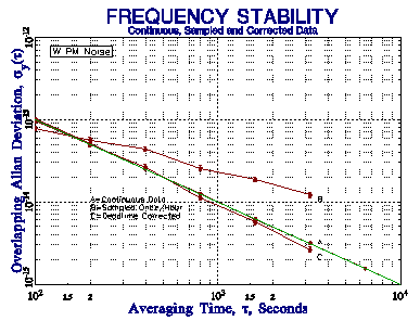
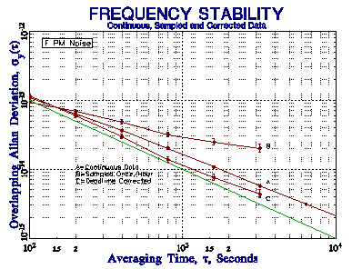
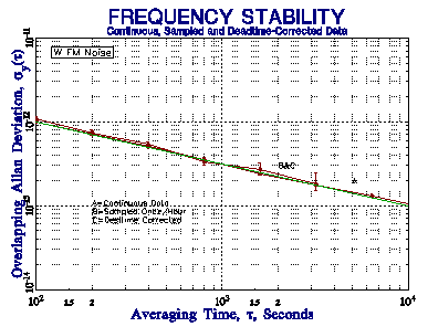
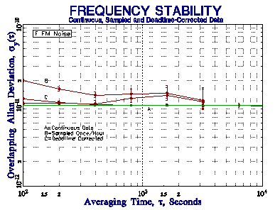
Dead time between measurements is quite common in frequency measurements, especially those made with an ordinary frequency counter. This may occur as the result of delay caused by the counter between successive measurements, or as the result of a deliberate wait between measurements. Because the latter can be quite long (e.g. one t = 100 second measurement made once per hour), it can have a significant effect on the results. Dead time that occurs at the end of a measurement can be adjusted for in an Allan deviation determination by using the Barnes B2 bias function [1], the ratio of the 2-sample variance with dead time ratio r = T/t to the 2-sample variance without dead time. Otherwise, without this correction, one can only determine the average frequency and its drift. When such data are used to form frequency averages at longer tau, it is necessary to also use the B3 bias function [2], the ratio of the variance with distributed dead time to the variance with all the dead time at the end. Those bias corrections are made using the product of B2 and B3. The power law noise type must be known in order to calculate these bias functions. Simulated periodically sampled frequency data with distributed dead time for various power law noise processes shows significant bias without, and good agreement with, the B2 and B3 bias function corrections, as shown in the figures below.
| Frequency
Stability Plots for Common Power Law Noises with Large Measurement Dead Time (r
= T/t = 36) Simulated Data Sampled for
t = 100 Seconds Once Per Hour for 10 Days Nominal 1x10-11 Stability at t = 100 Seconds Shown by Green Lines Plots Show Stability of Simulated Data Sets for Continuous, Sampled and Dead Time-Corrected Data |
|
 |
 |
| Figure 1. White PM (m = -2) ÖB2 = 0.82 at AF = 1 | Figure 2. Flicker PM (m = -2) ÖB2 = 0.82 at AF = 1 |
 |
 |
| Figure 3. White FM (m = -1) ÖB2 = 1.00 at AF = 1 | Figure 4. Flicker FM (m = 0) ÖB2 = 1.92 at AF = 1 |
 |
|
| Figure 5. RW FM (m = 1) ÖB2 = 7.31 at AF = 1 | |
These simulations show that the B2 and B3 bias corrections are able to support reasonably accurate results for sampled frequency stability data having a large dead time when the power law noise type is known. The slope of the raw sampled stability plot does not readily identify the noise type, however, and mixed noise types would make correction difficult. The relatively small number of data points reduces the confidence of the results, and limits the allowable averaging factor. Moreover, the infrequent measurements provide no information about the behavior of the clock during the dead time, and prevent a proper frequency to phase conversion. We therefore do not recommend using sparsely sampled data for the purpose of stability analysis. Nevertheless, should the need arise, Stable32 includes provisions for applying dead time corrections to its Sigma and Run Allan deviation estimates for known noise types.
MEASUREMENT SYSTEMS
In general, it is preferable to make continuous zero dead time phase measurements at regular intervals, and a system using a dual-mixer time interval measurement is recommended. An automated high-resolution multi-channel clock (phase) measuring system with a high-performance (e.g. hydrogen maser) reference is a major investment, but one that can pay off in better productivity. It is desirable that the measurement control, data storage, and analysis functions be separated to provide robustness and multiple network access to the data. A low-noise reference not only supports better measurement precision but also allows measurements to be made faster (with less averaging time). Stable32 can read and analyze stability data from essentially any measuring system.
TIMETAG FORMAT
Timetags are highly desirable for frequency stability measurements, particularly for identifying exact time of some anomaly. The preferred timetag is the Modified Julian Date (MJD) expressed as a decimal fraction and referenced to UTC. It is widely used, purely numeric, can have any required resolution, is easily converted to other formats, is non-ambiguous over a 2-century (1900-2099) range, and is free from seasonal (daylight saving time) discontinuities. Stable32 includes provisions for applying an offset to the timetags as they are read, which can be used to make time zone corrections or convert numeric Excel® dates to MJD. Stable32 also includes provisions for using MJD timetags, including convenient conversions to other common time and date formats.
DENOTING GAPS
Gaps in phase or frequency data can be denoted by a value of zero. This convention, while not entirely satisfactory, is an intuitive and effective choice. Zero is a simple value to enter and test for; the test can be either numeric or logical. For fractional frequency data, an actual value of zero can be approximated by some small value (e.g. 1e-99), which applies equally to any point. For phase data, it is quite likely that the first and last values are actually zero, so such points are not treated as gaps, and only imbedded zeros are considered gaps in phase data. As for frequency data, a small non-zero value can represent an actual phase values of zero. Frequency zeros may occur as the result of conversion from phase data having two equal adjacent values. This is most likely to happen for phase data of limited resolution for a stable, syntonized source. Small non-zero frequency values should be used for those cases. Because Stable32 uses a zero value to denote a gap, it has provisions for substituting 1e-99 for fractional frequency values of zero arising from equal adjacent phase measurements.
HANDLING GAPS
Stable32 includes a full set of editing, conversion, preprocessing, plotting and analysis functions be available that are capable of handling gaps. The editing tools are capable of finding, inserting and deleting gaps, and means are available for filling gaps with interpolated values. Phase-frequency conversion proceed smoothly through gaps. For conversion from fractional frequency to phase, the average frequency value is used for the interpolation. Plots show gaps as such, not connected by lines. Each analysis function includes specific means to handle gaps gracefully (e.g. second difference statistics ignore data where either point is missing).
VARIANCE CALCULATIONS WITH GAPS
Gaps in phase or frequency data may be skipped, filled, omitted, or excluded from variance calculations depending on whether the calculation is carried out with the gaps in the data, replaced with estimated values, removed from the data, or the calculation stopped at the gap. The basic objective is to be able to make a meaningful stability estimate even though the data set has missing points. Each of these approaches has advantages and disadvantages, and all of them alter the results to some extent compared with the same data set without gaps. Stable32 can perform some of its variance calculations with data that has gaps, but, in other cases, no reasonable algorithm exists for doing so, either because of the complexity involved, or because of the impact that gap handling has on computational speed. In that case, gaps are automatically filled as part of the variance calculation. A summary of the gap handling in the Stable32 variance functions (as of Version 1.46e) is shown in the table below, which applies to both phase and frequency data - in some cases, frequency data is automatically converted to phase data for the calculation .
| Stable32 Variance Function Gap Handling | ||
| Variance Type | Gap Handling | Gap Filling |
| Allan | X | |
| Overlapping Allan | X | |
| Modified Allan | X | |
| Time | X | |
| Hadamard | X | |
| Overlapping Hadamard | X | |
| Total Allan | X | |
| Total Modified | X | |
| Total Time | X | |
| Total Hadamard | X | |
| Thêo1 | X | |
| ThêoH | X | |
| TIE rms | X | |
| MTIE | X | |
Omitting gaps before the variance calculation changes the time flow of the data, but nevertheless may be the best approach, especially for a long group of contiguous gaps, which would be particularly unsuited to filling via linear interpolation. The calculation algorithm then does not have to handle gaps, and is therefore simpler and faster. Most importantly, no fictitious values are used that can change the noise properties of the data. That approach can be implemented by manually editing the data set before the calculation. Finally, one can simply stop the variance calculation at the gap by truncating the data set, or dividing it into sections. This would be particularly appropriate where the gaps occur near the beginning or end of the data. The integrity of the data is preserved, but the smaller number of analysis points will reduce the confidence in the result. In all cases, in is important that the analyst document the approach taken in handling gaps, so that the results are understood, and can be reproduced if necessary. Insight into gap handling can be gained by artificially introducing gaps into actual or simulated data, and processing it in different ways. The response of different analysis methods depends on the underlying noise type, the number and distribution of the gaps, and the type of variance used. It is recommended that such a study be conducted for any important data set that has more than a few percent of gaps. As an example, consider an overlapping Allan deviation analysis of the 1000-point FREQ.DAT white FM noise frequency data set distributed with Stable32. A utility program was written to substitute gaps (zeros) at random into a selectable percentage of this data set, and the resulting data files (with 1, 2, 5, 10, 20, 25, 33, or 50% gaps) were analyzed both with the gaps unfilled and filled. For those interested in duplicating this methodology, a data point was replaced with a gap according to the following test:
if(((i%10)-((int)(rand()*10.0/RAND_MAX)))==0)
where i is the data point index, and the 10's correspond to 10% gaps (on average). The rand() function is re-seeded for each run, which is repeated until the desired exact number of gaps is obtained. The results of this simulation study are shown below as all tau overlapping Allan deviation stability plots, and tables of the numeric results at octave averaging factors. The major conclusions are (1) acceptable results are obtained for 10% unfilled random gaps and 5% filled random gaps, and (2) gap filling by linear interpolation can significantly change the character of the white FM noise. It is interesting to consider filling gaps with estimated data based on the properties of the underlying noise. For example, for white FM noise, it would be better to fill gaps in frequency data with uncorrelated random values (of appropriate amplitude) rather than highly-correlated linearly interpolated ones. But one has to be careful not to get carried away by generating too much fictitious data. If your data has so many gaps that they, and the analysis details, start to have a significant impact on the results, it is better to fix the measurement problem that causes them rather than to manipulate the analysis.
| Overlapping Allan Deviation for Various Percentages of Random Gaps in Frequency Data | ||||||||
| AF | 1 | 2 | 3 | 4 | 5 | 6 | 7 | 8 |
| % Gaps | ||||||||
| 0 | 2.922 | 2.010 | 1.448 | 1.057 | 0.619 | 0.481 | 0.362 | 0.277 |
| 1 | 2.901 | 2.005 | 1.459 | 1.056 | 0.603 | 0.475 | 0.361 | 0.295 |
| 2 | 2.913 | 1.998 | 1.418 | 1.017 | 0.600 | 0.482 | 0.382 | 0.273 |
| 5 | 2.942 | 2.009 | 1.425 | 0.982 | 0.594 | 0.492 | 0.370 | 0.261 |
| 10 | 2.931 | 1.938 | 1.431 | 1.034 | 0.582 | 0.455 | 0.346 | 0.210 |
| 20 | 2.865 | 1.905 | 1.355 | 0.973 | 0.550 | 0.427 | 0.324 | 0.278 |
| 25 | 2.953 | 1.894 | 1.314 | 0.972 | 0.541 | 0.396 | 0.316 | 0.230 |
| 33 | 2.900 | 1.874 | 1.350 | 0.848 | 0.506 | 0.433 | 0.262 | 0.214 |
| 50 | 2.842 | 1.767 | 1.060 | 0.756 | 0.464 | 0.308 | 0.249 | - |
| Note | All sigma values in table multiplied by 10 for clarity | |||||||
These results are quite acceptable for up to 10% random gaps in the frequency data. Even for 50%, the results are remarkably good at the shorter averaging factors. The results are increasingly biased low as both the gap percentage and averaging factor increase, with a sigma value about half of normal with 50% gaps at the longest averaging factor. Even with that extreme number of gaps, the data still provides a good indication of the stability. In all cases, the stability plot generally follows the correct noise slope.
| Overlapping Allan Deviation for Various Percentages of Filled Gaps in Frequency Data | ||||||||
| AF | 1 | 2 | 3 | 4 | 5 | 6 | 7 | 8 |
| % Gaps | ||||||||
| 0 | 2.922 | 2.010 | 1.448 | 1.057 | 0.619 | 0.481 | 0.362 | 0.277 |
| 1 | 2.883 | 2.013 | 1.467 | 1.058 | 0.614 | 0.486 | 0.361 | 0.304 |
| 2 | 2.883 | 2.001 | 1.433 | 1.055 | 0.616 | 0.501 | 0.397 | 0.292 |
| 5 | 2.818 | 2.020 | 1.463 | 1.061 | 0.628 | 0.508 | 0.387 | 0.278 |
| 10 | 2.680 | 1.969 | 1.507 | 1.154 | 0.680 | 0.536 | 0.388 | 0.236 |
| 20 | 2.453 | 1.958 | 1.556 | 1.211 | 0.726 | 0.573 | 0.470 | 0.419 |
| 25 | 2.311 | 1.954 | 1.607 | 1.289 | 0.781 | 0.575 | 0.440 | 0.326 |
| 33 | 2.179 | 1.935 | 1.591 | 1.178 | 0.832 | 0.641 | 0.373 | 0.230 |
| 50 | 1.727 | 1.780 | 1.738 | 1.452 | 1.044 | 0.806 | 0.597 | 0.388 |
| Notes | All sigma values in
table multiplied by 10 for clarity Gaps filled by linear interpolation between adjacent points |
|||||||
The results are clearly worse for filled gaps. Not only are the sigma values in poorer agreement with the gap-free figures than those for unfilled gaps, but the stability plot slopes are also affected more. For filled data, the random gap limit for acceptable results is about 5%. The additional filled analysis points do, however, reduce the scatter in the results. Interestingly, the results tend to be biased high as the gap percentage and averaging factor increases. The poor results from the interpolated values is particularly pronounced for the larger gap percentages where there are more multiple contiguous gaps, and linear interpolation is a poor substitute for the underlying white FM noise.
UNEVEN SPACING
Unevenly spaced phase data can be handled if it has associated timetags by using the individual timetag spacing when converting it to frequency data. Then, if the tau differences are reasonably small, the data may be analyzed by using the average timetag spacing as the analysis tau. Stable32 includes provisions for handling irregularly spaced data in this way, in effect placing the frequency data on an average uniform grid. While completely random data spacing is not amenable to this process, tau variations of ±10% or so will yield reasonable results as long as the exact interval is used for phase to frequency conversion.
TWSTFT DATA
Two-way satellite time and frequency transfer (TWSTFT) data is an example of unevenly spaced data that is difficult to analyze. TWSTFT data is commonly taken once per day for three days (Monday, Wednesday, and Friday) per week. While these data are taken regularly, their spacing is uneven. A simulation of TWSTFT data and its time deviation (TDEV) analysis is shown in the plots below.
| TDEV Plots for TWSTFT Data | |
 |
 |
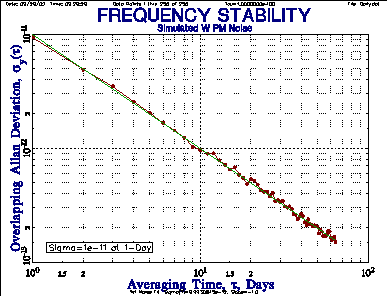
| Figure 6. ADEV Plot Actual sy(t) Very Close to Nominal Value |
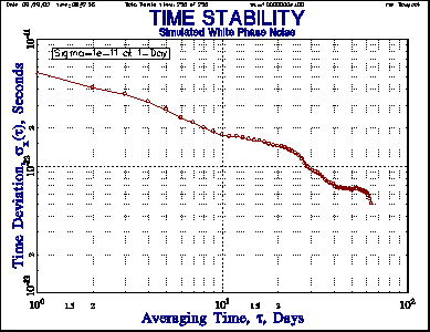
Figure 7. TDEV Plot Expected sx(t) = 5.77x10⁻¹² sec at t=1 Day |
| 256 Points of Simulated White FM Data with sy(t=1 Day) = 1x10-11 | |
 |
 |
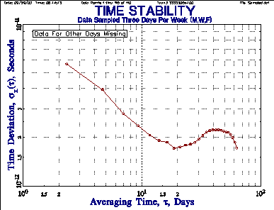
| Figure 8. Data Sampled for Three Days
Per Week (M, W, F) with Other Days Missing |
Figure 9. Sampled Data with Gaps
Inserted for Missing Data Points |
 |
 |
| Figure 10. Sampled Data with Missing
Points Filled by Linear Interpolation |
Figure 11. Sampled Data Converted to
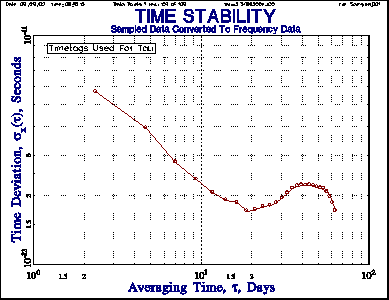
Frequency Data Using Timetags as Tau |
 |
|
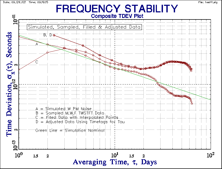
| Figure 12. Composite TDEV Plot | |
The simulated TWSTFT data is 256 points of white PM noise with an Allan deviation (ADEV) level of sy(t) = 1x10-11 at 1-day, as shown in Figure 6. Note that this, and all other stability plots, include points at all possible tau values. Figure 7 shows that the corresponding TDEV is 5.77x10⁻¹² sec at t=1 day (TDEV = MDEV divided by Ö3). The slope of the TDEV plot for W PM noise should be -0.5. The actual TWSTFT data is sampled once on Monday, Wednesday and Friday of each week. This sampled data therefore has an average tau of 7/3 = 2.33 days, and its TDEV is analyzed in Figure 8. If the missing points are included as gaps in the data, the resulting TDEV is shown in Figure 9. The erratic behavior is caused by interference between the tau and the gap periodicity. If the missing points are replaced by linearly interpolated phase values, the TDEV becomes highly distorted as shown in Figure 10. If the sampled phase data is converted to frequency data using their timetag differences to determine the individual measurement intervals, the average tau, tavg, is close to 2.33 days (depending on the final fractional week that is included), and the resulting TDEV is shown in Figure 11. It is essentially identical to that for the sampled phase data shown in Figure 8. It is interesting that, although the converted frequency results are different depending on whether the average or individual (more correct) taus are used, the (integrated) TDEV results are not (at least for a white PM noise process).
A composite plot of the TWSTFT TDEV results is shown in Figure 7. None of the results is in good agreement with the nominal simulation. The result with the linearly interpolated phase points is particularly bad, and is similar to that of Tavella and Leonardi as shown in Figure 1 of Reference [3]. As they point out in that paper, because the true sampling interval is tavg, it is not possible to estimate the noise at shorter times, especially for an uncorrelated white noise process. They further suggest that the higher level of the estimated noise is related to the ratio of the true and interpolated sampling times (»2.33) and the Öt dependence of TDEV. By applying a correction factor of Ö2.33 »1.5, the longer-tau TDEV estimates are lowered to the correct level. These factors are smaller for other non-white PM and FM noise processes. Hackman and Parker [4] suggest a set of correction factors for this type of unevenly-spaced data.
With Stable32, the adjusted method of using frequency data converted from phase data by using individual tau values adjusted for the timetag spacing is recommended because it does not use interpolation, does not present results at unrealistically low tau, and utilizes the best frequency estimates.
PARSIMONY
In any measurement or analysis, it is desirable to minimize the number of extraneous parameters. This is not just a matter of elegance; the additional parameters may be implicit or arbitrary and thereby cause confusion or error if they are ignored or misunderstood. For example, the Allan deviation has the important advantage that, because of its convergence characteristics for all common clock noises, its expected value is independent of the number of data points. Many of the techniques used in the analysis of frequency stability, however, do require that certain parameters be chosen before they can be performed. For example, drift removal requires the choice of a model to which the data will be fit (perhaps using the criterion of white residuals). Outlier removal is an especially difficult case, where judgment often enters into the decision as to whether or not a data point is anomalous. A listing of some of these non-parsimonious parameters is given in the table below.
| Table I. Non-Parsimonious Parameters in Frequency Stability Analysis | ||||
| Type | Process | Parameter | Criterion | Remarks |
| Preprocessing | Outlier removal | # of sigmas | Apply best judgment | Use of MAD-based robust statistics is recommended |
| Drift removal | To remove or not? |
Is drift deterministic? Is its cause known? | It is generally wise to remove deterministic drift before noise analysis | |
| Model | White residuals are a sign that the model is appropriate. | The model may have physical basis (e.g. diffusion process) | ||
| Convergence limit | For iterative fit | Generally uncritical - hidden deeply in fit algorithm | ||
| Remove average frequency | Model | Noise type | Not necessarily simple arithmetic mean of frequency | |
| Phase to frequency conversion | Tau | Accuracy | Is measurement interval known exactly? Is it the same for each point? | |
| Frequency to phase conversion | Tau | See above | ||
| Initial phase | Set to zero | Generally arbitrary -doesn't affect subsequent stability analysis | ||
| Normalize frequency | Use to emphasize noise rather than frequency offset | See "Remove average frequency" above | ||
| Analysis | Drift estimation | Model | White residuals | See "Drift removal" above |
| Convergence limit | For iterative fit | |||
| Frequency estimation | Model | Noise type | See "Remove average frequency" above | |
| Gaps | Skip, fill, omit, or exclude | Number, distribution, noise type | See "Variance Calculations with Gaps" above | |
| Allan deviation |
# data points | Confidence | Tradeoff against measurement time | |
| Dead time | Bias | Avoid if possible, otherwise correct for it | ||
| Maximum AF | Confidence | Generally biased low | ||
| Noise ID method to support error bars | Confidence | Needed to determine equivalent # of degrees of freedom | ||
| Hadamard deviation | All Allan deviation parameters | See above | ||
| Use rather than Allan deviation or separate drift removal? | Easier handling of clock with drift | Commonly used in GPS control operations | ||
| Total deviation | All Allan deviation parameters | See above | ||
| Use rather than Allan deviation? | Better confidence at long tau | Less common, longer computation time | ||
| Noise ID method to support bias removal | Both accuracy and confidence | Must apply bias correction based on noise type | ||
| Spectral analysis | Type - Parametric or non-parametric | Purpose | Non-parametric type more common | |
| Windowing - Bias reduction | Accuracy | Necessary | ||
| Smoothing - variance reduction | Confidence | Desirable | ||
| Presentation - plot or fit | Purpose | Usually plot | ||
| Presentation | Form | Table vs. Plot | Purpose | Both useful |
| Domain |
Time or frequency |
Purpose | Both useful and complementary | |
| Error bars | Include or not | Clarity | Error bars recommended | |
| Reference noise subtraction | Apply? | Accuracy | Used when reference stability is inadequate | |
| Nominal vs. maximum at some confidence level | Purpose | Confidence | Nominal value generally used. Tight confidence limit requires large data set. | |
| Notation | State outlier & drift removal, environmental conditions, etc. | Clarity | All pertinent conditions and analysis parameters should be documented | |
REFERENCES
Gaps.htm
10/19/06